November 18, 2019

hackseq

hackseq is a Vancouver-based hackathon focused on genomics. They want to bring individuals with diverse backgrounds together to collaborate on scientific questions and problems in genomics.

Their philosophy is open-source, open-notebook, open science.

Source: https://www.hackseq.com

Project Goals

Bioinformatics: the development and use of computational methods in genetics and genomics

Graphic Visualization of trends in Bioinformatics

  1. Usage of bioinformatic tools and technqiues (ex. sequence alignment, genome assembly, metagenomics etc)
  2. Relationship of tool development within analytical pipelines
  3. Geographic hotspots for development of bioinformatic tools and techniques

End product: A visualization tool of trends in Bioinformatics, which can help prospective graduate students choose an institution or area of research.

Source: http://tiny.cc/hs19-readme

Trends in Bioinformatics

Analogy

Field Topic Search Terms
Bioinformatics Sequencing Sanger, next-generation sequencing, …
Bioinformatics Assembly Short read assembly, long read assembly, …
Fruits Apples Ambrosia, Gala, McIntosh, Granny Smith, …
Fruits Oranges Navel, Mandarin, Tangerine, Clementine, …

Webscraping Results

Dataframe:

## # A tibble: 12 x 4
##    db        found searchTerm           topic     
##    <chr>     <dbl> <chr>                <chr>     
##  1 plos       9554 sanger sequencing    Sequencing
##  2 bmc       48995 sanger sequencing    Sequencing
##  3 crossref  37023 sanger sequencing    Sequencing
##  4 entrez    96509 sanger sequencing    Sequencing
##  5 arxiv     54228 sanger sequencing    Sequencing
##  6 scopus    89260 sanger sequencing    Sequencing
##  7 plos      34911 long read sequencing Sequencing
##  8 bmc      324406 long read sequencing Sequencing
##  9 crossref 434845 long read sequencing Sequencing
## 10 entrez   339648 long read sequencing Sequencing
## 11 arxiv    145774 long read sequencing Sequencing
## 12 scopus    39175 long read sequencing Sequencing

Webscraping Results

Our Dataset

Let’s look at the search terms of one specific topic, one specific jounral:

Sequencing in the Public Library of Science (PLoS)

## # A tibble: 10 x 9
##    doi    journal  publisher  author1  affiliation  title  abstract  topic  Year
##    <chr>  <chr>    <chr>      <chr>    <chr>        <chr>  <chr>     <chr> <dbl>
##  1 10.13… PLoS ONE Public Li… Zaragoz… Genetics & … Mitoc… Mutation… sang…  2010
##  2 10.13… PLoS ONE Public Li… Ji, Hez… National HI… HIV D… Backgrou… sang…  2010
##  3 10.13… PLOS ONE Public Li… Landria… Department … Inher… Spinocer… sang…  2017
##  4 10.13… PLOS ONE Public Li… Guinois… INSERM U966… Deep … Hepatiti… sang…  2017
##  5 10.13… PLOS ONE Public Li… Iyer, S… Department … Compa… Massivel… sang…  2015
##  6 10.13… PLOS ONE Public Li… Rebolle… Department … Compa… The refe… sang…  2015
##  7 10.13… PLOS ONE Public Li… Vivien,… Swiss Centr… Next-… Aquatic … sang…  2016
##  8 10.13… PLOS ONE Public Li… Pandey,… AIT Austria… MutAi… Traditio… sang…  2016
##  9 10.13… PLoS ONE Public Li… Lopez-R… Laboratorio… Compa… Backgrou… sang…  2012
## 10 10.13… PLoS ONE Public Li… Shokral… Biodiversit… Pyros… DNA barc… sang…  2011
To follow along with some live-coding, download these worksheets:
http://tiny.cc/rladies-ws1
http://tiny.cc/rladies-ws2

Racing Bar Graph

What is a Racing Bar Graph?

What is a Racing Bar Graph?

Regular Bar Graph

First, let’s load our dataset and make a regular bar graph:

base <- "https://raw.githubusercontent.com/dy-lin/hs19-trends/master/workshop/"
seq_spec <- "data/sequencing-specific-processed.csv"
url <- paste0(base, seq_spec)
seq_data <- read_csv(url)

A glimpse into the dataset (top 5):

topic Year total cum_total
illumina 2013 171 404
capillary 2013 153 495
sanger 2013 152 406
illumina 2014 142 546
10x genomics 2015 141 525

Regular Bar Graph

reg <- seq_data %>%
  drop_na() %>%
  ggplot(aes(x = topic, y = cum_total, fill = topic)) +
  geom_col() + 
  facet_wrap(~ Year, ncol = 8) + 
  coord_flip() +
  scale_fill_viridis_d() +
  theme(axis.text.y = element_blank(),
        axis.ticks.y = element_blank(),
        legend.position = "bottom") +
  geom_text(aes(y = cum_total, 
                label = topic), 
            hjust = "left", 
            fontface = "bold", 
            nudge_y = 50)

Regular Bar Graph

Racing Bar Graph

In order to make a racing bar chart, where the bars overtake one another, we need to rank the topics for each year:

ordered_df <- NULL

for (yr in 2003:2019) {
  order <- seq_data %>% 
    filter(Year == yr) %>% 
    arrange(cum_total) %>% 
    mutate(ordering = row_number())
  
  ordered_df <- ordered_df %>% rbind(order)
}

Racing Bar Graph

Here’s what the dataset looks like now:

topic Year total cum_total ordering
10x genomics 2004 1 1 1
capillary 2004 2 2 2
next-generation 2005 1 1 1
sanger 2005 1 1 2
capillary 2005 2 4 3
oxford nanopore 2006 1 1 1
10x genomics 2006 1 2 2
next-generation 2006 4 5 3
sanger 2006 5 6 4

Racing Bar Graph

Here is an overview of the code:

# plot
p <- ordered_df %>% 
  ggplot(aes(ordering, group = topic)) +
  geom_col(aes(y = cum_total, width = 0.9, fill = topic)) +
  geom_text(aes(y = cum_total, label = topic), 
            hjust = "left", fontface = "bold", nudge_y = 50) +
  coord_cartesian(clip = "off", expand = FALSE) +
  scale_fill_viridis_d() +
  coord_flip() +
# animate
  transition_states(Year, transition_length = 8, state_length = 4, wrap = FALSE) +
  ease_aes("cubic-in-out") +
# aesthetics
  labs(subtitle = "Trends in sequencing methods", title = "Year {closest_state}", 
       y = "cumulative total papers") +
  theme(plot.background = element_blank(), legend.position = "none",
        axis.ticks.y = element_blank(), axis.text.y = element_blank(),
        text = element_text(size=14), plot.title = element_text(size = 35)) +
  ylim(0,1300) +
  xlab("") 

Racing Bar Graph

Let’s start plotting:

# plot
p <- ordered_df %>% 
  ggplot(aes(ordering, group = topic)) +
  geom_col(aes(y = cum_total, width = 0.9, fill = topic)) +
  geom_text(aes(y = cum_total, label = topic), 
            hjust = "left", fontface = "bold", nudge_y = 50) +
  coord_cartesian(clip = "off", expand = FALSE) +
  scale_fill_viridis_d() +
  coord_flip() +
# animate
  transition_states(Year, transition_length = 8, state_length = 4, wrap = FALSE) +
  ease_aes("cubic-in-out") +
# aesthetics
  labs(subtitle = "Trends in sequencing methods", title = "Year {closest_state}", 
       y = "cumulative total papers") +
  theme(plot.background = element_blank(), legend.position = "none",
        axis.ticks.y = element_blank(), axis.text.y = element_blank(),
        text = element_text(size=14), plot.title = element_text(size = 35)) +
  ylim(0,1300) +
  xlab("") 

Racing Bar Graph

coord_cartesian(clip = "off", expand = FALSE)

Usage:

coord_cartesian(xlim = NULL, ylim = NULL, expand = TRUE, default = FALSE, clip = "on")

Description:

The Cartesian coordinate system is the most familiar, and common, type of coordinate system. Setting limits on the coordinate system will zoom the plot (like you’re looking at it with a magnifying glass), and will not change the underlying data like setting limits on a scale will.

Arguments

  • expand: If TRUE, the default, adds a small expansion factor to the limits to ensure that data and axes don’t overlap. If FALSE, limits are taken exactly from the data or xlim/ylim.
  • clip: Should drawing be clipped to the extent of the plot panel? A setting of “on” (the default) means yes, and a setting of “off” means no. In most cases, the default of “on” should not be changed, as setting clip = “off” can cause unexpected results. It allows drawing of data points anywhere on the plot, including in the plot margins.

Racing Bar Graph

Next, to set up some animation parameters:

# plot
p <- ordered_df %>% 
  ggplot(aes(ordering, group = topic)) +
  geom_col(aes(y = cum_total, width = 0.9, fill = topic)) +
  geom_text(aes(y = cum_total, label = topic), 
            hjust = "left", fontface = "bold", nudge_y = 50) +
  coord_cartesian(clip = "off", expand = FALSE) +
  scale_fill_viridis_d() +
  coord_flip() +
# animate
  transition_states(Year, transition_length = 8, 
                    state_length = 4, wrap = FALSE) +
  ease_aes("cubic-in-out") +
# aesthetics
  labs(subtitle = "Trends in sequencing methods", y = "cumulative total papers",
       title = "Year {closest_state}") +
  theme(plot.background = element_blank(), legend.position = "none",
        axis.ticks.y = element_blank(), axis.text.y = element_blank(),
        text = element_text(size=14), plot.title = element_text(size = 35)) +
  ylim(0,1300) +
  xlab("") 

Racing Bar Graph

transition_states(Year, transition_length = 8, state_length = 4, wrap = FALSE)

Usage:

transition_states(states, transition_length = 1, state_length = 1, wrap = TRUE)

Description:

This transition splits your data into multiple states based on the levels in a given column, much like ggplot2::facet_wrap() splits up the data in multiple panels. It then tweens between the defined states and pauses at each state.

Arguments:

  • states: The unquoted name of the column holding the state levels in the data.
  • transition_length: The relative length of the transition. Will be recycled to match the number of states in the data
  • state_length: The relative length of the pause at the states. Will be recycled to match the number of states in the data
  • wrap: Should the animation wrap-around? If TRUE the last state will be transitioned into the first.

Racing Bar Graph

ease_aes("cubic-in-out")

Usage:

ease_aes(default = "linear", ...)

Description:

Easing defines how a value change to another during tweening. Will it progress linearly, or maybe start slowly and then build up momentum. In gganimate, each aesthetic or computed variable can be tweened with individual easing functions using the ease_aes() function. All easing functions implemented in tweenr are available, see tweenr::display_ease for an overview. Setting an ease for x and/or y will also affect the other related positional aesthetics (e.g. xmin, yend, etc).

Functions

  • cubic: Models a power-of-3 function
  • -in-out: The first half of the transition it is applied as-is, while in the last half it is reversed

Racing Bar Graph

Lastly, set up some aesthetics:

# plot
p <- ordered_df %>% 
  ggplot(aes(ordering, group = topic)) +
  geom_col(aes(y = cum_total, width = 0.9, fill = topic)) +
  geom_text(aes(y = cum_total, label = topic), 
            hjust = "left", fontface = "bold", nudge_y = 50) +
  coord_cartesian(clip = "off", expand = FALSE) +
  scale_fill_viridis_d() +
  coord_flip() +
# animate
  transition_states(Year, transition_length = 8, state_length = 4, wrap = FALSE) +
  ease_aes("cubic-in-out") +
# aesthetics
  labs(subtitle = "Trends in sequencing methods", 
       title = "Year {closest_state}", y = "cumulative total papers") +
  theme(plot.background = element_blank(), legend.position = "none",
        axis.ticks.y = element_blank(), axis.text.y = element_blank(),
        text = element_text(size=14), plot.title = element_text(size = 35)) +
  ylim(0,1300) +
  xlab("") 

Racing Bar Graph

Let’s animate!

The figure shown on the next slide was generated using these parameters:

# render the animation
animate(p, nframes = 750, fps = 20, end_pause = 10)

However, due to the lengthy time it takes to generate, we should reduce these numbers:

# rendering the animation
animate(p, nframes = 100, fps = 5, end_pause = 10)

Racing Bar Graph

animate(p, nframes = 100, fps = 5, end_pause = 10)

Usage:

animate(plot, ...)

Description:

This function takes a gganim object and renders it into an animation. The nature of the animation is dependent on the renderer, but defaults to using gifski to render it to a gif. The length and framerate is decided on render time and can be any two combination of nframes, fps, and duration. Rendering is happening in discrete time units.

Arguments

  • plot: A gganim object
  • nframes: The number of frames to render (default 100)
  • fps: The framerate of the animation in frames/sec (default 10)
  • duration: The length of the animation in seconds (unset by default)
  • start_pause,end_pause: Number of times to repeat the first and last frame in the animation (default is 0 for both)

Racing Bar Graph

Sankey Diagrams

What is a Sankey Diagram?

Sankey Diagrams

Here are the packages we need to load for a Sankey diagram:

library(tidyverse)
library(ggrepel)
library(grid)
library(ggalluvial)
library(egg)

Sankey Diagram

Let’s load in our pre-processed dataset:

base <- "https://raw.githubusercontent.com/dy-lin/hs19-trends/master/workshop/"
SK <- "data/sankey-processed.csv"
url <- paste0(base, SK)
datSK <- read_csv(url)
From To Weight count
EMBL Databases 14 26
Harvard U Phylogenetics 12 19
U Washington Variant Calling 10 25
Baylor College of Medicine Variant Calling 10 26
UC San Diego Genome Annotation 8 17
U Michigan Phylogenetics 8 16

Sankey Diagram

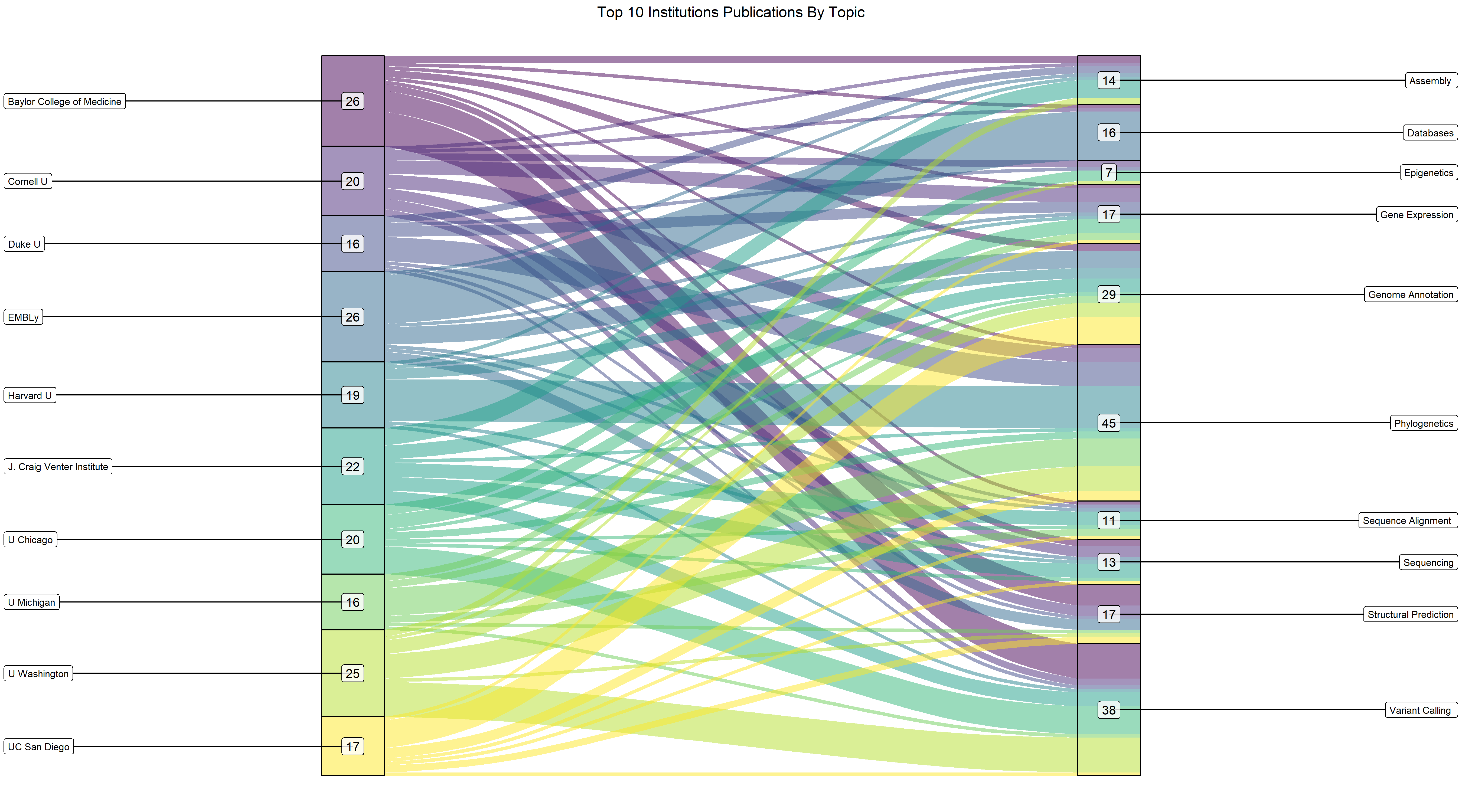
Here’s an overview of plotting the Sankey diagram using ggplot:

sankey <- ggplot(datSK, aes(y = Weight, axis1 = From, axis2 = To)) +
  geom_alluvium(aes(fill = From), width = 1 / 12) +
  geom_stratum(alpha = 0, width = 1 / 12, color = "black") +
  scale_x_discrete(limits = c("From", "To"), expand = c(0.3, 0.1)) +
  scale_fill_viridis_d() +
  theme_void() +
  theme(axis.title.y = element_blank(), axis.title.x = element_blank(),
    axis.ticks.x = element_blank(), axis.ticks.y = element_blank(),
    axis.text.x = element_blank(),axis.text.y = element_blank(),
    legend.position = "none", plot.title = element_text(hjust = 0.5)) +
  ggrepel::geom_label_repel(
    aes(label = From), stat = "stratum", size = 3, direction = "x", hjust = 10) +
  ggrepel::geom_label_repel(
    aes(label = To), stat = "stratum", size = 3, direction = "y", nudge_x = 0.5) +
  geom_label(aes(label = Weight), stat = "stratum", alpha = 0.8) +
  ggtitle("Top 10 Institutions Publications By Topic")

sankey <- set_panel_size(sankey, width  = unit(18, "cm"), height = unit(10, "cm"))
grid.newpage()
grid.draw(sankey)

Sankey Diagram

Let’s take a closer look at the geom functions used:

sankey <- ggplot(datSK, aes(y = Weight, axis1 = From, axis2 = To)) +
  geom_alluvium(aes(fill = From), width = 1 / 12) +
  geom_stratum(alpha = 0, width = 1 / 12, color = "black") +
  scale_x_discrete(limits = c("From", "To"), expand = c(0.3, 0.1)) +
  scale_fill_viridis_d() +
  theme_void() +
  theme(axis.title.y = element_blank(), axis.title.x = element_blank(),
    axis.ticks.x = element_blank(), axis.ticks.y = element_blank(),
    axis.text.x = element_blank(),axis.text.y = element_blank(),
    legend.position = "none", plot.title = element_text(hjust = 0.5)) +
  ggrepel::geom_label_repel(
    aes(label = From), stat = "stratum", size = 3, direction = "x", hjust = 10) +
  ggrepel::geom_label_repel(
    aes(label = To), stat = "stratum", size = 3, direction = "y", nudge_x = 0.5) +
  geom_label(aes(label = Weight), stat = "stratum", alpha = 0.8) +
  ggtitle("Top 10 Institutions Publications By Topic")

sankey <- set_panel_size(sankey, width  = unit(18, "cm"), height = unit(10, "cm"))
grid.newpage()
grid.draw(sankey)

Sankey Diagram

geom_alluvium(aes(fill = From), width = 1 / 12)

Usage:

geom_alluvium(mapping = NULL, data = NULL, stat = "alluvium", position = "identity", width = 1/3, knot.pos = 1/6, na.rm = FALSE, show.legend = NA, inherit.aes = TRUE, ...)

Description:

geom_alluvium receives a dataset of the horizontal (x) and vertical (y, ymin, ymax) positions of the lodes of an alluvial diagram, the intersections of the alluvia with the strata. It plots both the lodes themselves, using geom_lode(), and the flows between them, using geom_flow().

Arguments:

  • mapping: Set of aesthetic mappings created by aes()
  • width: Numeric; the width of each stratum, as a proportion of the distance between axes. Defaults to 1/3.

Sankey Diagram

geom_stratum(alpha = 0, width = 1 / 12, color = "black")

Usage:

geom_stratum(mapping = NULL, data = NULL, stat = "stratum", position = "identity", show.legend = NA, inherit.aes = TRUE, width = 1/3, na.rm = FALSE, ...)

Description:

geom_stratum receives a dataset of the horizontal (x) and vertical (y, ymin, ymax) positions of the strata of an alluvial diagram. It plots rectangles for these strata of a provided width.

Arguments:

  • width: Numeric; the width of each stratum, as a proportion of the distance between axes. Defaults to 1/3.

Sankey Diagram

Mapping

Mapping

We want to look at several trends

  • Most Common topic per country
  • Number of papers per country


If you still haven’t downloaded the live-coding worksheet for this section:
http://tiny.cc/rladies-ws2

Mapping

Mapping

Here are all the packages we need to format the data and do the plotting

library(ggplot2)
library(dplyr)
library(plotly)
library(here)
library(ggmap)
library(viridis)
library(rgeos)
library(maptools)
library(maps)
library(sf)
library(readr)
library(tidyverse)
library(knitr)
library(broom)

Mapping

Packages needed for plotting

ggplot2: package for data visualizations

plotly: makes interactive visualizations

viridis: good colour palatte for dealing with colourblindness and greyscale issues

Mapping

There is a lot of code in the worksheet that describes how we got the data into the format we needed

  • We will do one global plot and one of Europe

Mapping

Here is an example of what the data looks like:

long lat group order region subregion Count topicMax
14572 -61.10518 45.94472 252 14823 Canada Cape Breton Island 616 transcript quantification
14573 -61.07134 45.93711 252 14824 Canada Cape Breton Island 616 transcript quantification
14574 -60.93657 45.98555 252 14825 Canada Cape Breton Island 616 transcript quantification
14575 -60.86524 45.98350 252 14826 Canada Cape Breton Island 616 transcript quantification
14576 -60.86840 45.94863 252 14827 Canada Cape Breton Island 616 transcript quantification
14577 -60.98428 45.91069 252 14828 Canada Cape Breton Island 616 transcript quantification
14578 -61.03755 45.88222 252 14829 Canada Cape Breton Island 616 transcript quantification
14579 -60.97060 45.85581 252 14830 Canada Cape Breton Island 616 transcript quantification
14580 -60.97153 45.83799 252 14831 Canada Cape Breton Island 616 transcript quantification

Mapping

pl <- ggplot() +
  geom_polygon(data = world_data2, aes(x = long, y = lat,
  group = group,fill = log(Count),text=Count),colour="lightgrey") +
  coord_fixed(1.3)+
  scale_fill_viridis()+
  theme_void()

world_plotly=ggplotly(pl,tooltip = "text")

Mapping

geom_polygon(data = world_data2, aes(x = long, y = lat,group = group,fill = log(Count),text=Count))

Usage

geom_polygon:mapping = NULL, data = NULL, stat = "identity",position = "identity", rule = "evenodd", ..., na.rm = FALSE,show.legend = NA, inherit.aes = TRUE)

Description

Polygons are very similar to paths (as drawn by geom_path()) except that the start and end points are connected and the inside is coloured by fill. The group aesthetic determines which cases are connected together into a polygon.

Arguments

group:By default, the group is set to the interaction of all discrete variables in the plot. This often partitions the data correctly, but when it does not, or when no discrete variable is used in the plot, you will need to explicitly define the grouping structure, by mapping group to a variable that has a different value for each group.

Mapping

pl <- ggplot() +
  geom_polygon(data = world_data2, aes(x = long, y = lat,
  group = group,fill = log(Count),text=Count)) +
  coord_fixed(1.3)+
  scale_fill_viridis()+
  theme_void()

world_plotly=ggplotly(pl,tooltip = "text")

Mapping

Mapping

If we want to look at certain countries we can do that too

  • depending on how much data is in one region this may be a good idea
  • will have to figure out the coordinates you want
  • plot will be set up similarily to the global one but we will add in new elements

Mapping

X region Count long lat group order subregion
67 67 Albania 0 19.96484 39.87227 6 836 NA
68 68 Albania 0 19.85186 40.04356 6 837 NA
69 69 Albania 0 19.48457 40.20996 6 838 NA
70 70 Albania 0 19.39814 40.28486 6 839 NA
71 71 Albania 0 19.36016 40.34771 6 840 NA
72 72 Albania 0 19.32227 40.40708 6 841 NA

Mapping

 pl <- ggplot() + 
  geom_polygon(data = europe_data, aes(x = long, y = lat, 
  group = group, fill = log(Count),
  text=paste(region,Count, sep=";"))) +
  geom_point(data=points_europe,aes(x=X,y=Y,
  text=str_wrap(affiliation,50)),
  alpha=0.5,size=0.5,colour="grey")+
  coord_fixed(1.3)+
  scale_fill_viridis()+
  theme_void()

Mapping

Bigrams

Bigrams

Bigrams are two consecutive words within a given text input

  • ex. We love coding in R
  • (We Love), (Love coding), (coding in), (in R)

Bigrams

library(tidyverse)
library(tidytext)
library(tm)
library(widyr)
library(igraph)
library(ggplot2)
library(ggraph)
library(readr)
library(tidygraph)

Bigrams

ggraph: visualizations for network structures

ggplot2: package for data visualizations

Bigrams

visualize_bigrams: extracts bigrams from a text field, calculates frequency of bigrams, and creates a bigram plot to visualize relationships between words

  • df_name: name of dataframe that contains the text field of interest
  • textfield: name of text field (ie. column name)
visualize_bigrams <- function(df_name, textfield, topic_title)

Bigrams

In the worksheet, you will see a lot of code that just talks about the formatting of the data. If you are interested in that look into it, but we’re just covering the plotting

Bigrams

pl <- graph_hold %>%
      ggraph(layout = "fr") +
      geom_edge_link(aes(edge_alpha = Edge_Frequency),
      show.legend = TRUE) +
      geom_node_point(aes(color = Term_Frequency, 
      size = Term_Frequency), alpha = 0.7) +
      scale_fill_viridis_c() +
      geom_node_text(aes(label = name), repel = TRUE) +
      scale_color_viridis_c(direction = -1) +
      theme_void() +
      guides(size=FALSE) +
      labs(title = quo_name(topic_title)) +
      theme(plot.title = element_text(size = 26, face = "bold"))

Bigrams

geom_edge_link(aes(edge_alpha = Edge_Frequency),show.legend = TRUE)

Usage

geom_edge_link(mapping = NULL, data = get_edges("short"),position = "identity", arrow = NULL, n = 100, lineend = "butt",linejoin = "round", linemitre = 1, label_colour = "black",label_alpha = 1, label_parse =FALSE, check_overlap = FALSE,angle_calc = "rot", force_flip = TRUE, label_dodge = NULL,label_push = NULL, show.legend = NA, ...)

Description

This geom draws edges in the simplest way - as straight lines between the start and end nodes. Not much more to say about that…

Bigrams

ggraph(layout = "fr")

Usage

ggraph(graph, layout = "auto", ...)

Description

This function is the equivalent of ggplot2::ggplot() in ggplot2. It takes care of setting up the plot object along with creating the layout for the plot based on the graph and the specification passed in. Alternatively a layout can be prepared in advance using create_layout and passed as the data argument.

Arguments

layout:The type of layout to create. Either a valid string, a function, a matrix, or a data.frame

  • fr is within the igraph layout options for constucting node diagrams

Bigrams

geom_node_point(aes(color = Term_Frequency, size = Term_Frequency), alpha = 0.7)

Usage

geom_node_point: geom_node_point(mapping = NULL, data = NULL, position = "identity",show.legend = NA, ...)

Description

This geom is equivalent in functionality to ggplot2::geom_point() and allows for simple plotting of nodes in different shapes, colours and sizes.

Arguments

We don’t use any arguments in this case, just change some of the aes

Bigrams

## 
## 
## |Search Term           |
## |:---------------------|
## |Assembly              |
## |Databases             |
## |Epigenetics           |
## |Gene Expression       |
## |Genome Annotation     |
## |Phylogenetics         |
## |Sequence Alignment    |
## |Sequencing            |
## |Structural Prediction |
## |Variant Calling       |

Bigrams

df_assembly <- df %>% 
  filter(topic == "Assembly")
visualize_bigrams(df_assembly, abstract, "")

Bigrams

GitHub

Acknowledgements

  • Jasmine Lai
  • Raissa Philibert
  • Lucia Darrow
  • Shannon Lo
  • Morgana Xu
  • Elliot YKF
  • Swapna Menon


Thank you RLadies and Dialpad for hosting us!